About lasagne, splitting methods and your favourite film
The ‘Divide and Conquer’-principle was already used in the Roman foreign policy. The politicians and warlords of the ancient world noticed that a large group of people can be easier controlled or even conquered if you split them up into several smaller groups.
Quicksort algorithm: source
CC BY-SA3.0 Roland H.
Luckily the ancient times are long gone, but the principle remains, in particular in computer science. Many algorithms are based on the idea of splitting a task into several easy-to-handle parts. After solving these simpler parts, the solution of the full problem needs to be reconstructed from the solutions of these subproblems. So, it is possible to ‘conquer’ a complex task.
A famous example is the well-known Quicksort algorithm to sort a list of numbers. You start by picking one number in the list (the pivot element) and compare it to every other number of the list. If the other number is smaller, we put it on the left side of our pivot element, if it is larger, we put it on the right side. Thus, we get two sublists, one with smaller and one with larger numbers than the pivot element. We continue to sort these sublists in the same way with new pivot numbers from the sublists. The complete list is sorted when all sublists are sorted.
You may wonder what this is all about and how this is related to our CRC?
We are interested in solving differential equations. A differential equation usually serves as a simplified model for a complex physical process. The heat equation for example describes the temperature distribution in a metal plate and the wave equation models the propagation of optical pulses in media, for instance. For many problems one can prove, that unique solutions exist, but unfortunately, explicit formulas for the exact solutions of such equations usually do not exist. A numerical method computes an approximation to the solution, which helps physicists and engineers in their understanding of the processes. There is a widely used class of numerical methods called splitting methods. These methods in particular rely on the ‘Divide and Conquer’ principle. In our CRC we are using splitting methods and that’s why I would like to focus on them now. As a matter of fact, they were also a topic of our recent summer school.
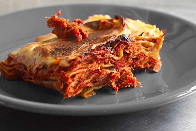
Lasagne, source, CC BY-SA2.0 Isabelle Palatin
In computer science splitting often helps to save computation time. For our numerical method it first of all helps to find an approximation to the solution at all. Sometimes it is even possible to compute the solution of the subproblems exactly, while the exact solution of the full problem is unknown. In order to understand this phenomenon, imagine someone starting to cook. A student, who already learned to prepare ragu and bechamel sauce but has never heard of lasagne or ate one, will not be able to produce a lasagne. But if someone tells him, how to split the problem ‘cooking a lasagne’ into the subproblems
- cook a ragu sauce,
- cook a bechamel sauce,
- stack in turns ragu, lasagne sheets and bechamel sauce in a casserole,
- scatter cheese on top,
- put it into the oven
which he can handle, he will be able to cook a lasagne.
The main difference is that in mathematics, we are often not able to compute the exact solution of the problem, even if we can solve all subproblems exactly. While a lasagne recipt can be splitted into several tasks and the lasagne is a combination of their solutions, the interactions between the subproblems often gets lost when a differential equation is splitted. Think of cooking the ragu sauce. You can detect two effects while heating the pot. Firstly the sauce at the bottom gets warmer and secondly the heat of the lower layer of the sauce spreads into the upper layers. If we split these two physical processes as for a splitting method, the combination as an approximation of the heating effect could be
- heat the lower layer,
- spread the heat in the upper layers.
Since, however, in reality the two effects happen simultaneously, the combination by successively solving the subproblems misses this permanent interaction. So the approximation will not be exact.
As a second difference our lasagne-recipe consists of a fixed (and small) number of different steps to complete the cooking process. For a splitting method we usually have only two or three different subproblems, but we will not only solve them once. Instead we will combine their solutions to an approximation after a small time step and then we will iteratively apply this solution several times to get a good approximation on a larger time interval. But what does that actually mean?
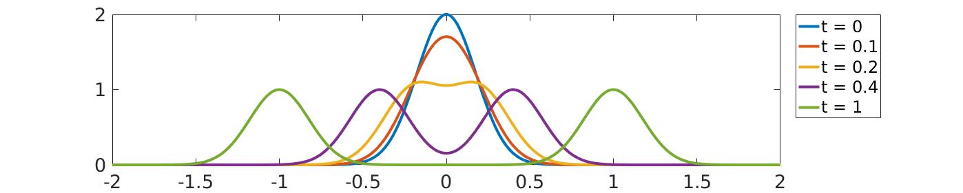
Wave propagating in space from x = -2 to x = 2 at different times t
In the picture above we can see a wave, which travels in space over time. Usually we are interested in the solution (here the shape of the wave) at a fixed time. For our wave we know the shape of the wave at some initial time 0 (initial value) and we may want to know how the wave looks like at a later time 1. In general, we will not compute an approximation by just applying our numerical method once with one large time step. Instead we will typically apply the method several times with a smaller step size. Therefore we use the recently computed approximation to a previous time step as a new initial value for the next time step. In the case of the wave, we compute an approximation to the shape of the wave at time 0.1 and take this shape as a new initial value to compute the approximated shape of the wave at time 0.2. After 10 such steps we would have an approximation to the shape of the wave at time 1.
This may seem complicated, but the reason for this procedure is simple: the numerical approximation gets better if a smaller step size is used. To illustrate this phenomenon, lets think of your favorite film. As you may already know a film consists of single frames. The frames are stacked in a row and you see every frame just a very short time. So there is a specific time step between two frames while in reality the movement is continuous. If we would decrease this time step the resulting film shows judder. Thus, we see that the size of the time step has to be small enough, that the film is a good approximation to reality.

Our Logo in different resolutions
In addition, the frames in the film consist of millions of pixels. A pixel represents the color information of a tiny part of the frame. The frame has a high resolution, if the number of pixel is so large that our human eye is not able to differentiate between the single colored dots and will show us a continuous picture. But if we decrease the number of pixels, i.e. use larger pixels, we will loose details and the image starts to blur (you can see this in the picture above where we reduced the pixels in our logo). So while the time difference between two frames in a film represents the time step size, the length of a pixel in a single frame represents the spatial step size. Hopefully, this explains why it is not a good idea to represent a film by a single frame with a single pixel.
Naturally, the question arises whether the numerical method is able to compute the exact solution if the step size gets smaller and smaller. The answer is yes on one hand while it is no on the other. Usually, the task of a mathematician working on numerical analysis is to prove that the error between a numerical solution and the exact solution tends to zero if the step size tends to zero. This shows that the method is reasonable (it converges) and it is also possible to characterize the ‘quality’ of a method (for experts, the order of accuracy). So, yes, the approximation should get better, if we take a smaller step size. However in practice, the computational effort rises if we choose a smaller step size, since we simply have to perform more intermediate steps to get the desired result. Often it is not feasible to reduce the step size beyond a certain level, but usually, the achieved accuracy is sufficient for the actual application. So, yes, we can get close to the exact solution, but we will not be able to compute it.
The aim of our CRC is to unite analysis and numerics. The example of splitting methods shows what that means and why this is so important. We talked about ‘solving the subproblems’. For this task researchers in the field of analysis are needed. They provide exact solutions to the subproblems and help us to find properties of the exact solution, which allows to construct a good numerical method. However, even more important for numerical mathematicians, analytical mathematicians are often able to show that the problem is solvable, i.e. that a unique exact solution exists (even if there is no explicit expression for it). This is a necessary condition for the error analysis of a numerical method, so for analysing the quality of a numerical method. In the end, numerical mathematicians try to implement their methods efficiently on a computer. So, you can see, these fields of mathematics are closely linked.
Let us explain this connection using the lasagne example. First in analysis, mathematicians will prove, that lasagne exist. The lasagne is a picture for the solution of a differential equation, so we now know, that our lasagne exists and fulfills some equation, but we are not able to construct a lasagne explicitly. Like if we have a picture of the lasagne, but we do not know the recipe. Then numerical mathematicians detect the subproblems by considering the equation, so for the lasagne they will study the picture and detect some kind of noodle plates, ragu and bechamel sauce. In a next step, researches in analysis may be able to construct explicit solutions to these subproblems, like recipes to cook the sauces. In addition they may know more properties of the exact solution, which then helps numerical researches to construct a good splitting method to approximate it. An important property of the lasagne is, that it consists of several layers of noodles. In math, qualitative properties of solutions could be energy or mass conservation (e.g. of a physical or chemical process). The construction of a splitting method consists of a suitable combination of the solutions of the subproblems, like writing a recipe, how to approximatively cook lasagne. Here, the properties of the solution are important to obtain a good approximation. We can imagine that if we lack enough information we might get cannelloni instead of lasagne.
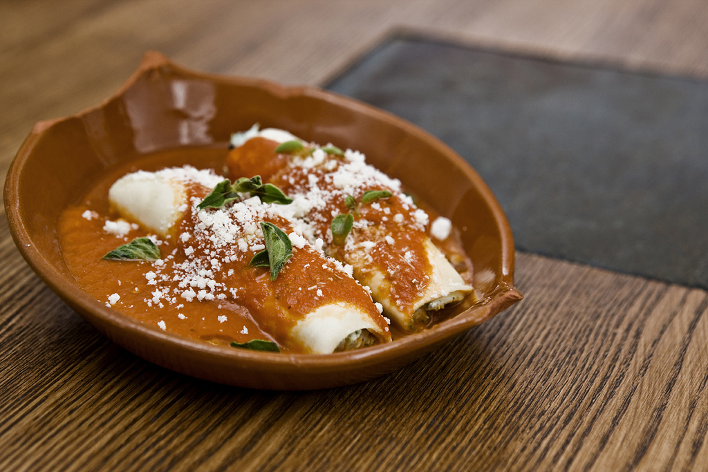
Cannelloni,
source,
CCBY-NC2.0 by Bottega
In the previous sections we learned that in contrast to a cooking recipe, a numerical method consists of an algorithm to construct a solution on a small time interval and afterwards we apply this algorithm iteratively for many time steps to get a solution on a larger time interval. Finally, numerical mathematicians will analyze the quality of this new method by comparing the result of our approximated recipe with the original lasagne. And they will find an efficient implementation, so for the lasagne this could be an instruction how to cook it very fast and with as few cooks as possible.
I hope this article provides an inside view on splitting methods and the work of mathematicians in general. Splitting methods are famous in the numerical community, because they provide a way to create new efficient methods for complex problems by using already existing, fully tested solutions to simpler tasks. In addition there usually exist very efficient implementations of the solutions of the subproblems, and thus the implementation of a splitting method is simple and convenient. So the ancient ‘Divide and Conquer’ principle is relevant more then ever. In our CRC splitting methods are considered in many projects. Publications and preprints can be found here (see for example 3, 4, 19 and 22 of 2016). For a mathematical introduction to splitting methods I recommend the ‘yellow book’ Geometric Numerical Integration by E. Hairer, C. Lubich and G. Wanner.
At the end, I would like to thank Marlis Hochbruck, Johannes Eilinghoff, Piotr Idzik, Lena Martin and Patrick Krämer for proof-reading and helpful discussions during the writing process of this article.