In the following I would like to present the main ideas of bifurcation theory along with some basic examples that illustrate the theory. For the sake of shortness let me formulate the fundamental question of bifurcation theory in an abstract way. Suppose you are given an equation \(F(x,\lambda)=0\) with the property that \(x=0\) is always a solution, the so-called trivial solution. Is it possible to find some \(\lambda^*\) such that a sequence of nontrivial solutions converges to \((0,\lambda^*)\)? In other words: Do nontrivial solutions bifurcate from the trivial solutions? In the following I will present three equations from analysis, linear algebra and ordinary differential equations showing that bifurcation theory is a topic worth studying! The reading requires some amount of advanced mathematics — do not hesitate to contact me if you need some additional explanations. By the way: Next semester I will give a lecture on that topic which is suited for master students or advanced bachelor students with a background in analysis, differential equations and possibly boundary value problems, see below for more information.
Example 1
Consider the equation $$ \lambda x – x^3 = 0$$ where \(x,\lambda\) are real numbers. This equation has the feature that the trivial solution is always a solution, but there are nontrivial solutions as well! Factoring \(x\) out we find that all nontrivial solutions satisfy \(\lambda=x^2\). Hence we observe that nontrivial solutions bifurcate from \(\lambda^*=0\) which may be illustrated as follows:
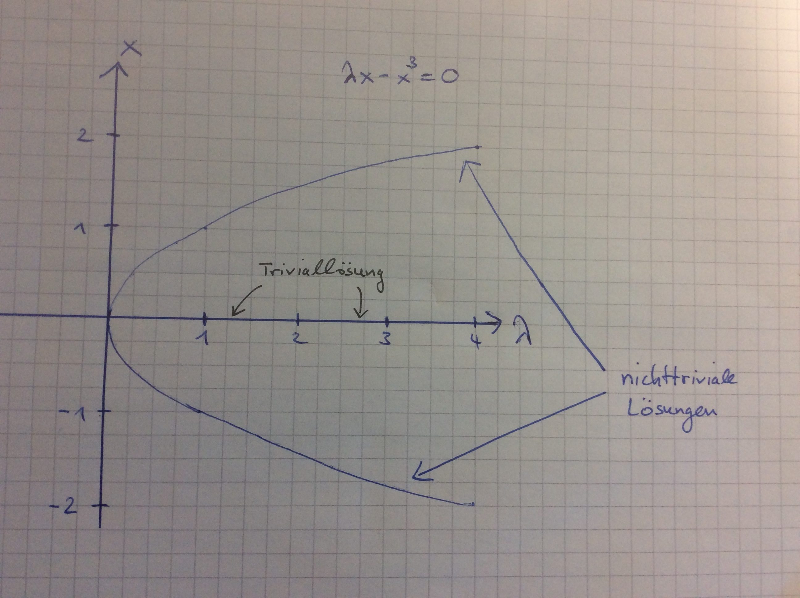
Here it is comparatively easy to illustrate all solutions and the above picture, a so-called bifurcation diagram, shows why we speak of bifurcations. Notice that the latin word furca means fork (Gabel in German) so that a literal translation of bifurcation to German language would be Zweigabelung. However, mathematicians say Verzweigung. The reader may amuse him-/herself by replacing the exponent 3 by 4: How does the picture change?
Example 2
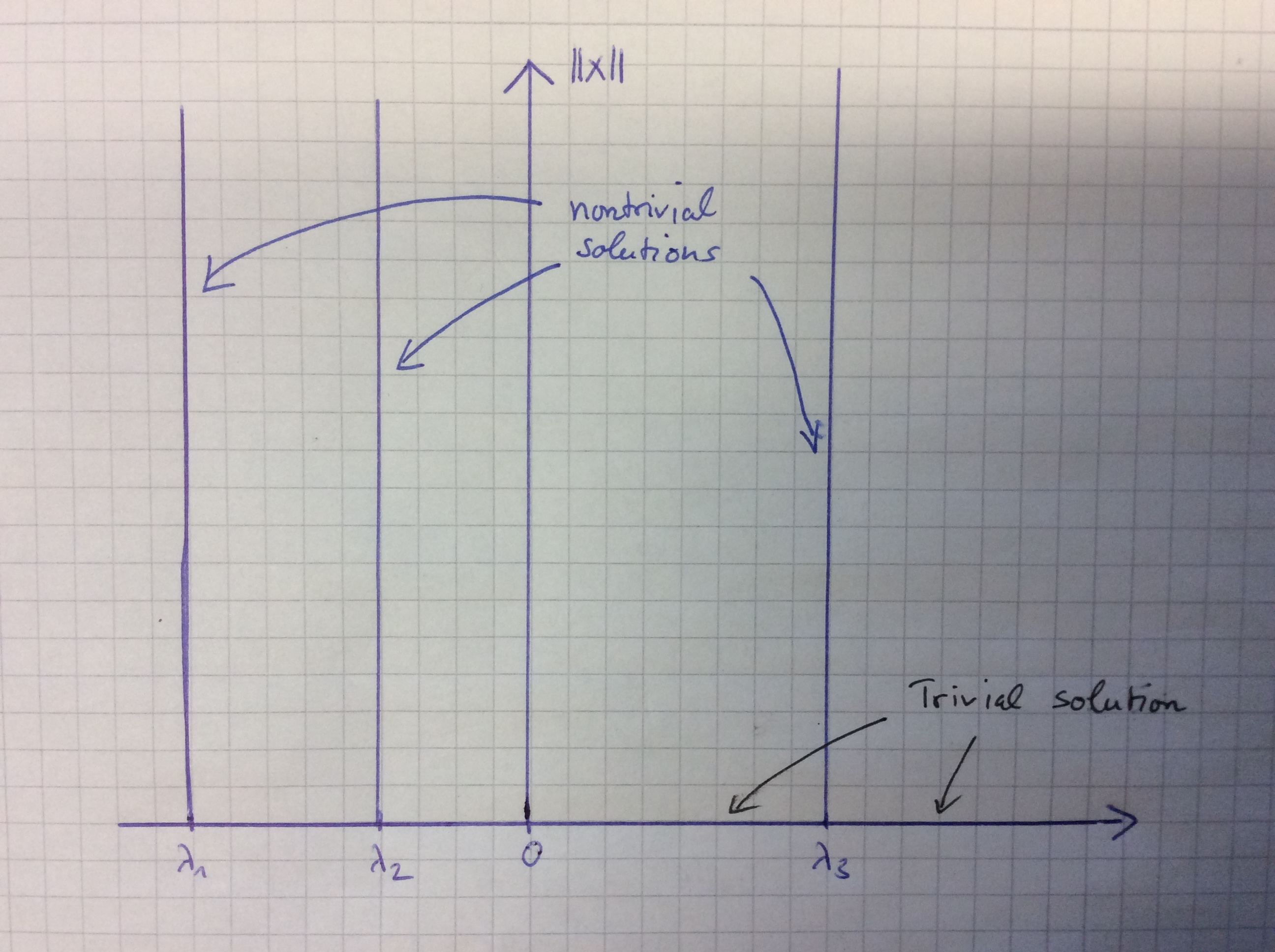
The next equation represents one of the fundamental problems of linear algebra: Which are the eigenvalues of a given quadratic matrix \(A\)? In other words: Find the nontrivial solutions \((\lambda,x)\) of the equation $$ Ax – \lambda x=0.$$ After two semesters of linear algebra the solution is pretty clear: If \(\lambda\) is a real eigenvalue of the matrix then it is a bifurcation point. More precisely, if the geometric multiplicity is bigger than 2 then there is even a surface of nontrivial solutions (spanned by the eigenvectors) that bifurcates from the trivial solution. The bifurcation diagram below illustrates the case of 3 simple eigenvalues.
Example 1 and 2 show that the phenomenon occurs, but we have to clarify why it is worth a theory if we can calculate all nontrivial solutions by hand? The simple answer to that question is that the above examples are artificial and made for expository purposes. In most applications from analysis we have to deal with nonlinear problems in infinite-dimensional (Banach) spaces. Here, it is in general impossible to calculate explicit solutions that bifurcate from the trivial solution so that one has to use some nontrivial tools from nonlinear analysis and functional analysis that allow to treat such a problem. Such tools can be used, e.g., for the study of boundary value problems for partial and ordinary differential equations.
Example 3
Finally, I would like to mention the pendulum equation $$\theta”(t) + \lambda \sin(\theta(t)) = 0,\qquad \theta(0)=\theta(T/2)=0.$$ Here \(\theta\) denotes the angle with respect to the vertical (rest) position and \(T\) is the oscillation period while the parameter lambda is proportional to the inverse of the length of the pendulum. In the first lectures of my course I will provide a method that allows to show that the bifurcation diagram is, qualitatively, the following:
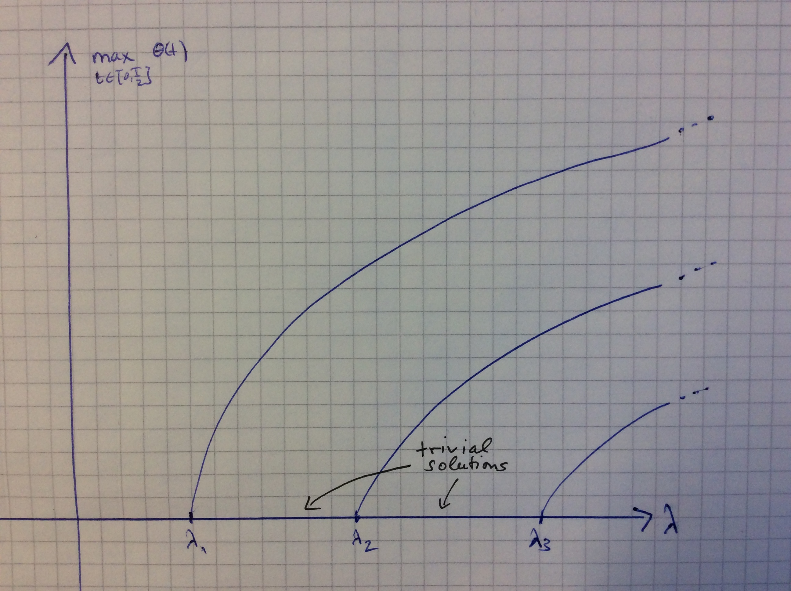
Every point on some curve corresponds to a solution of the above boundary value problem and the vertical component measures its maximum. In particular we see that for any preassigned period we get more and more oscillating solutions the larger \(\lambda\) is, i.e. the smaller the pendulum is. This matches our real-life experience, doesn’t it? Of course, a more realistic model should include friction effects and also such problems can be treated.
Lecture announcement
Next semester (summer term 2017) I will give a 2+2-course on Bifurcation theory where we will develop a functional analytical framework to study problems like the ones above and much more complicated ones. The topics will cover the Implicit Function Theorem in Banach spaces, bifurcation from a simple eigenvalue (Crandall–Rabinowitz Theorem), bifurcation from infinity, Hopf bifurcation for periodic solutions of ordinary differential equations. The prerequisites are a thorough knowledge of analysis, ordinary differential equations and the basics of functional analysis or boundary and eigenvalue problems.
In the winter term 2017/2018 I am going to offer two options to broaden your expertise in bifurcation theory. There will be a seminar based on the lecture and another lecture where topological methods and/or variational will be applied to bifurcation problems. These methods allow to detect so-called global bifurcations, which is much better but also much more advanced than the local bifurcations we find in the up-coming lecture. Either course can be a starting point for a master thesis.
Contact information: Rainer.Mandel@kit.edu